How to use sum function in MS excel | How to use auto sum in MS Excel 2016
How to use sum function in MS excel and How to use auto sum in MS Excel 2016 is equally beneficial for teachers as well as students.The Sum is most widely used operation in daily mathematics and accounting. Likewise, MS Excel has an extensive SUM function. With the aid of this function one can do various type arithmetic operations regarding SUM. Post Moreover, ease and simplicity is another good thing that facilitate user to use these formulas. How to use sum function in MS Excel post will train you to effectively use SUM function.
In addition to this you may find other related posts on our web. Which are as under:
Computer Trivia | MCQs with answer on CPU
History and Generation of Computer short essay
Basic Computer Quiz Questions With Answers
The benefits of using a word processor
How to insert header and footer in excel
Methods mentioned in this document support MS Excel XP and above versions like MS Excel 2007,2010,2011,2013, 2016.
Simply sum, multiply, divide and subtract operations can be done by giving ranges with following syntax:
=A7+A9+B8+B10
=A7*A9*B8*B10
=A7+A9/B8+B10
=A7+A9-B8+B10
SUM function is part of Math & Trig function of MS Excel. Following are part of this category:
SUM
SUMIF
SUMIFS
SUMPRODUCT
SUMSQ
SUMX2MY2
SUMX2PY2
SUMXMY2
Now one by one each of above functions are explained:
SUM function:
As explained above SUM function is part of Math & Trig category. Either you can you use individual data value or references data values for this function. Moreover, combination of both types can also applied.
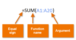
Syntax:
=SUM (number1, [number2],…)
Where number 1 is the first data value and number 2 is the second data value that you are going to add.
More precisely above syntax appears as
=SUM(A1:A12)
=SUM(A1:A12, C2:C10)
In above syntax A1 represents position of data value at intersection of column A and row 1. Similarly one can use multiple selection for summing more than one data ranges.
How to use sum function in MS excel
SUMIF function:
SUMIF function is also part of Math & Trig category. One can use individual data value or references data values for this function. While, combination of both types can also be used.
Syntax:
The syntax for the SUMIF function in Microsoft Excel is:
SUMIF( range, criteria, [sum_range] )
In above syntax, range of cells is that limit upto which you want to apply criteria. Criteria is used to determine which cells you want to add and sum range tells you to sum together.
=SUMIF(A5:A9, F3, C2:C6)
=SUMIF(B2:B6, “>=2012”, D2:D6)
Here criteria is greater and equal to 2012
SUMIFS function:
Sometime need arises to use multiple criteria rather using single criteria, in such cases you can use SUMIFS function which is also part of Math & Trig category. Similar to SUMIF individual data value as well as references data values for this function can be employed. While, combination of both types can also be used.
Syntax
The syntax for the SUMIFS function in Microsoft Excel is:
SUMIFS( sum_range, criteria_range1, criteria1, [criteria_range2, criteria2, …] )
SUMPRODUCT function:
SUMPRODUCT function multiplies corresponding values in (Arrays) rows or columns and it returns the sum of their respective product of rows or columns as given in the formula selection or range.
Syntax
SUMPRODUCT (array1, [array2], [array3], …)
The above items show:
• Array1: The collection of first rows and columns which you want to multiply.
• Array2: The collection of second rows and columns which you want to multiply.
=SUMPRODUCT (A4:B8, D5:E9)
The above formula will calculate the product of A4 to B8 data and will sum up to the product of data D5 to E9.
SUMSQ function:
It gives us sum of the squares of the data values or arguments.
Syntax
SUMSQ(number1, [number2], …)
In above syntax number 1 and number 2 are two arguments, the formula will calculate the square of both arguments and then it will sum to give result.
Simply =SUMSQ(2, 5) will give us answer 29
SUMX2MY2 function:
Its result will be the sum of the difference of squares of corresponding values in two given arrays.
It has following syntax:
=SUMX2MY2(Array 1, Array 2)
Instead of taking the time to click the Sum button on the Home tab, it’s often faster and easier to simply press Alt+= (equal sign) to insert the SUM function in the current cell and have Excel select the range of cells most likely to be totaled.
Reference : (colon) Range operator that includes =SUM(C4:D17)
, (comma) Union operator that combines multiple references
into one reference =SUM(A2,C4:D17,B3)
(space) Intersection operator that produces one reference to cells in common with two references
=SUM(C3:C6 C3:E6)
=AVERAGEIFS(data_range, criteria_range1, criteria1[,criteria_ range2, criteria2…]).
SUMIF Finds the sum of values in a range that meet a single criterion
The SUMIFS, AVERAGEIFS, and COUNTIFS functions extend the capabilities of the SUMIF,
AVERAGEIF, and COUNTIF functions to allow for multiple criteria. If you want to find the sum of all orders of at least $100,000 placed by companies in Washington, you can create the formula =SUMIFS(D2:D5, C2:C5, “=WA”, D2:D5, “>=100000”).
SUMIFS Finds the sum of values in a range that meet multiple criteria
=SUMIFS(F3:F14, C3:C14, “=Envelope”, E3:E14, “=International”),
Few Important points about SUMIF and SUMIFS Formulas:
Both SUMIF and SUMIFS formulae support wildcard characters. You can use wildcard characters (like: ‘*’ and ‘?’) in the ‘criteria’ argument.
Moreover, In SUMIF the cells in ‘range’ argument and ‘sum range’ need not be of same shape and size. But this does not stands true in case of SUMIFS.
You can use multiple operators (like: “=”, “>”, “<”, “>=”, “<=”, “<>”) in the ‘criteria’ argument of both the functions.
=SUMIFS(E3:E11,B3:B11,”West”,D3:D11,”>500″)
Notes:
To sum a column of numbers, select the cell immediately below the last number in the column. To sum a row of numbers, select the cell immediately to the right.
AutoSum is in two locations: Home > AutoSum, and Formulas > AutoSum.
Once, you create a formula, you can copy it to other cells instead of typing it over and over. For example, if you copy the formula in cell B7 to cell C7, the formula in C7 automatically adjusts to the new location, and calculates the numbers in C3:C6.
Moreover, You can also use AutoSum on more than one cell at a time. For example, you could highlight both cell B7 and C7, click AutoSum, and total both columns at the same time.
IMSUM function
Applies To: Excel 2016 Excel 2013 Excel 2010 Excel 2007 Excel 2016 for Mac More…
This article describes the formula syntax and usage of the IMSUM function in Microsoft Excel.
Description
Returns the sum of two or more complex numbers in x + yi or x + yj text format.
Syntax
IMSUM(inumber1, [inumber2], …)
The IMSUM function syntax has the following arguments:
Inumber1, [inumber2], … Inumber1 is required, subsequent numbers are not. 1 to 255 complex numbers to add.
Remarks
Use COMPLEX to convert real and imaginary coefficients into a complex number.
The sum of two complex numbers is: Equation
Example
First, copy the example data in the following table, and paste it in cell A1 of a new Excel worksheet. In the second phase for formulas to show results, select them, press F2, and then press Enter. If you need to, you can adjust the column widths to see all the data.
=IMSUM(“3+4i”,”5-3i”)
Sum of two complex numbers
8+i
SERIESSUM function
Applies To: Excel 2016 Excel 2013 Excel 2010 Excel 2007 Excel 2016 for Mac More…
This article describes the formula syntax and usage of the SERIESSUM function in Microsoft Excel.
Description
Many functions can be approximated by a power series expansion.
Returns the sum of a power series based on the formula:
Syntax
SERIESSUM(x, n, m, coefficients)
The SERIESSUM function syntax has the following arguments:
X Required. The input value to the power series.
N Required. The initial power to which you want to raise x.
M Required. The step by which to increase n for each term in the series.
Coefficients Required. A set of coefficients by which each successive power of x is multiplied. The number of values in coefficients determines the number of terms in the power series. For example, if there are three values in coefficients, then there will be three terms in the power series.
Remark
If any argument is nonnumeric, SERIESSUM returns the #VALUE! error value.
Example
At first, Copy the example data in the following table, and paste it in cell A1 of a new Excel worksheet. For formulas to show results, select them, press F2, and then press Enter. If you need to, you can adjust the column widths to see all the data.
Data
Coefficients as numbers
Coefficients as formulae
0.785398163
=PI()/4
1
1
-0.5
=-1/FACT(2)
0.041666667
=1/FACT(4)
-0.001388889
=-1/FACT(6)
=SERIESSUM(A3,0,2,A4:A7)
Approximation to the cosine of Pi/4 radians, or 45 degrees (0.707103)
0.707103
SUMPRODUCT function
Applies To: Excel 2016 Excel 2013 Excel 2010 Excel 2007 Excel 2016 for Mac More…
This article describes the formula syntax and usage of the SUMPRODUCT function in Microsoft Excel.
Description
Multiplies corresponding components in the given arrays, and returns the sum of those products.
Syntax
SUMPRODUCT(array1, [array2], [array3], …)
The SUMPRODUCT function syntax has the following arguments:
Array1 Required. The first array argument whose components you want to multiply and then add.
Array2, array3,… Optional. Array arguments 2 to 255 whose components you want to multiply and then add.
Remarks
The array arguments must have the same dimensions. If they do not, SUMPRODUCT returns the #VALUE! error value.
SUMPRODUCT treats array entries that are not numeric as if they were zeros.
Example
Copy the example data in the following table, and paste it in cell A1 of a new Excel worksheet. For formulas to show results, select them, press F2, and then press Enter. If you need to, you can adjust the column widths to see all the data.
Array 1 3 4 8 6 1 9
Array 2 2 7 6 7 5
=SUMPRODUCT(A2:B4, D2:E4)
Multiplies all the components of the two arrays and then adds the products — that is,
3*2 + 4*7 + 8*6 + 6*7 + 1*5 + 9*3 (156)
Result is 156
SUMSQ function
Applies To: Excel 2016 Excel 2013 Excel 2010 Excel 2007 Excel 2016 for Mac More…
This article describes the formula syntax and usage of the SUMSQ function in Microsoft Excel.
Description
Returns the sum of the squares of the arguments.
Syntax
SUMSQ(number1, [number2], …)
The SUMSQ function syntax has the following arguments:
Number1, number2, … Number1 is required, subsequent numbers are optional. 1 to 255 arguments for which you want the sum of the squares. You can also use a single array or a reference to an array instead of arguments separated by commas.
Remarks
Arguments can either be numbers or names, arrays, or references that contain numbers.
Moreover, numbers, logical values, and text representations of numbers that you type directly into the list of arguments are counted.
On the other hand, If an argument is an array or reference, only numbers in that array or reference are counted. Empty cells, logical values, text, or error values in the array or reference are ignored.
Arguments that are error values or text that cannot be translated into numbers cause errors.
Example
At first, copy the example data in the following table, and paste it in cell A1 of a new Excel worksheet. Secondly, For formulas to show results, select them, press F2, and then press Enter. If you need to, you can adjust the column widths to see all the data.
Formula
Description (Result)
Result
=SUMSQ(3, 4)
Sum of the squares of 3 and 4 (25)
25
Finally some more related tips and tricks for MS office are as mentioned:
The benefits of using a word processor
Microsoft office 2013 tutorial | Tips and tricks for Microsoft office 2013
How to insert header and footer in excel
we hope you enjoy-How to use sum function in MS excel | How to use auto sum in MS Excel 2016- please comments and subscribe our channel.
https://www.youtube.com/channel/UCDBixME-h0BQZG3GGU4FRiw

Pingback: Word experienced an error trying to open the file
only a few survived.